A brief overview to arrays and stacks

Faouzi Braza

2025-09-15

Beneath every line of code, every variable or every loop, there is a physical reality lying along in silicon: the Random Access Memory (RAM). And if you are going to write code, it helps to understand what is really happening down there. Array is a very neat data structure and quite easy to understand. It also allows us to understand quite simply what we are actually storing in RAM.

At the most fundamental level, we are storing information as bits, data that can be either 0 or 1. Eight of those bits form a byte. And when we talk about RAM like 8 gigabytes, we are talking about roughly 8 billion of those bytes, all lined up in one long, contiguous space of memory. (Technically, 1 GB = 10^9 bytes. But purists will whisper “but actually, it’s 2^30”. And they are not wrong. We will nod respectfully and keep moving.)

Now, when we store something like an integer, we are usually grabbing 4 bytes (sometimes more, if we need higher precision). That is 32 bits — 31 of them holding the number’s value, and one often keeping track of its sign (if the integer is signed). A character, by contrast, typically fits neatly into just 1 byte. Simple, right?

The Illusion of index and the reality of memory addresses

As programmers, we rarely think in terms of memory addresses. We use index. These are clean, human-friendly numbers like array[0], array[1], and so on. (Though if you have ever coded in R, you know the delightful rebellion of starting at 1. Be blessed R.)

But under the hood? Every index maps directly to a physical memory address. It is a specific location in that long space of RAM. And because arrays are stored contiguously, namely one value right after the next, we can compute any address instantly, given the starting point and the index. That is why reading from an array is a constant operation. In engineering language we often talk about time complexity and Big O notation. I am not a computer scientist by training. But keep in mind that the Big O notation is a good way to evaluate how much time the operation will cost. Accessing or reading value in an array is constant time or O(1). No matter how big the array grows, accessing array[1000000] takes the same time as array[0].

That is the “Random” in “Random Access Memory”. RAM is not chaotic, but freely navigable. A beautiful, engineered kind of freedom.

These type of concepts are not only theoretical. This actually allowed me to understand the concept behind pointers. A pointer is a variable that stores a memory address. And at that memory address we have a value.

Static arrays: simple, fast, and slightly stubborn

In languages like C, arrays are often static. This means they have a fixed in size from the moment you declare them. You allocate 10 slots? You get 10 slots. No more, no less. (Python and JavaScript, bless their dynamic hearts, hide this from us. But the reality underneath is still there. We discuss that in the next section)

With static arrays:

Reading any element? O(1).
Writing to an existing slot? Also O(1).
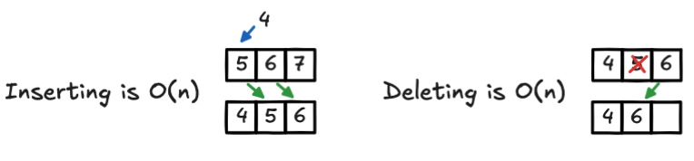
Adding or removing at the end? Still O(1), if you have space to add the value.
But inserting or removing from the middle? Now we are talking O(n).

Why `O(n)``? Simply because memory does not magically re-arrange itself.

Imagine you have an array [5, 6, 7] and you want to insert 4 at the beginning of this array. To make room, you need to shift everything over. Move 6 to index 2, 5 to index 1 and then slip 4 into index 0. Our array is [4, 5, 6]. 7 disappeared. To succeed we performed n operations. One for each element you shift out of the way. Same goes for deletion. Now we remove 5. Ok 6 has to shift back to fill the gap. Again: O(n). Our array is [4, 6].

Remember that static array has a finite space in memory. And manipulating this array by inserting or removing elements may take work.

Dynamic arrays: what happens when your array outgrows?

So, static arrays are tidy. They are predictable and somewhat rigid. A bit like suitcase you packed for a weekend trip and then suddenly decided to move across the country for a year.

Enter the dynamic arrays.

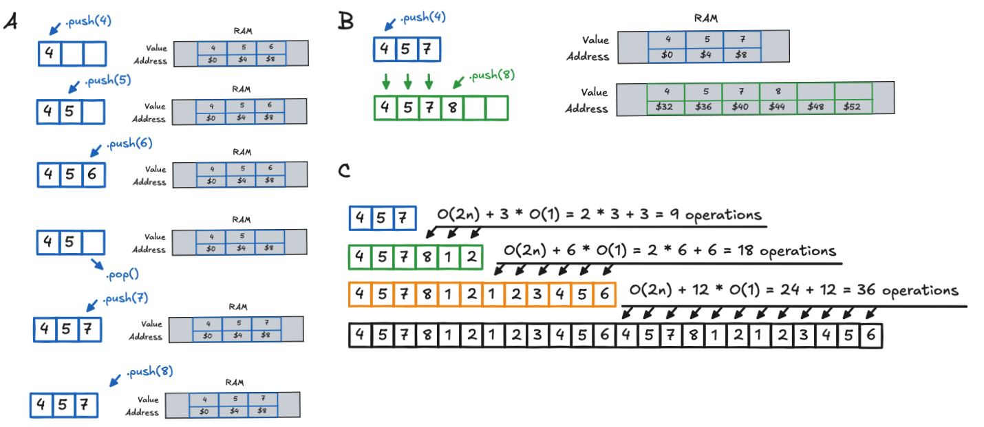
For programmers, notably in Ruby, Python or Javascript, dynamic arrays feel magical. In Python you can initialize an array as simply as my_array = []. In Scala, you have a specific type for dymnamic array ArrayBuffer[Int]() which quietly reserves 16 slots for you. In both cases these arrays will grow as you need them. Push a value? O(1). Pop one at the end? Also O(1).

💡 Note: you will see these operations called different things. For push it is .append() in Python, .push() in Ruby, or even += in Scala. Same thing but with different names.

The thing is that, even if the grow seems natural, a lot of things happen under the hood. Indeed RAM does not grow on trees. Arrays, even dynamic ones, still live in contiguous blocks of memory. That is what makes random access so fast. But when you run out of space, the machine cannot just “make new room.” It has to move to a new space and re-allocate new slots (see the figure 2).

The great array re-allocation

Imagine we start with a tiny array of size 3 and filled it up: [4, 5, 7]. Now you want to add 8. Here we reach a situation where we acutally have no space left. Indeed the memory address just next to our 3 slots could acutally be used by something else. The only way to add this new value will be to:

Let the system find a new, larger block of memory of size 4 for example.
Next, copy all your existing values over one by one. That is O(n).
Then add the new value, 8. That’s O(1).

The total cost? O(n) + O(1) = O(n).

(Big O, in its infinite wisdom does not care about constants. So O(2n)? Still O(n).)

Now imaging doing that every time you add an element. Arf. It is like repacking your entire suitcase every time you buy a new pair of socks. Clearly inefficient and unnecessary. A possibility could be to double the size instead of allocating only one additional slot. So when starting with 3 → next allocation is 6. Then 12. Then 24. As n grows, that expensive O(n) copy operation only happens occasionally. Most of the time, you are just slipping values into empty slots at O(1). We do “waste” some space but over time, the average cost per insertion stays constant. This is called amortized analysis / complexity.

📊 The math:
Let’s say copying costs 2n (find space + copy), and you get n new free slots. Total cost for n insertions: 2n. Average per insertion: 2n / n = 2 → which Big O rounds down to… O(1).
In our figure example:

(1) 3 → 6: cost = 9, avg = 3.

(2) 6 → 12: cost = 18, avg = 3.

(3) 12 → 24: cost = 36, avg = 3.
Cost is being constant.

One last thing. The re-allocation factor is flexible. That “doubling” thing is not an immutable law. It is just engineering. Some languages multiply by 1.5. Others use more complex heuristics. CPython, for example, does not quite double. It increases by a factor that is roughly 1.125x for smaller arrays, scaling up as needed.

From dynamic arrays to Stacks

Dynamic arrays do not just give us flexible storage. They also give us the foundation to build stacks. Stack is one beautiful yet simple idea.

“Last In, First Out.” Like a stack of plates. Or a browser’s back button. Or undoing your last three typos one by one, in reverse.

For stacks we do not need a new data structure. We just need discipline. With a dynamic array, you enforce two rules:

You only add (push) to the end.
You only remove (pop) from the end.

And That is it. No inserting in the middle. No random access. No shuffling. The usual operations found with stacks are the following:

Operation	Description	Time Complexity
`.push(item)`	Add an item to the top	O(1) amortized
`.pop()`	Remove and return top item	O(1)
`.peek()`	View top item (no removal)	O(1)
`.is_empty()`	Check if stack has no items	O(1)

And because we are only touching the end + the amortized O(1), everything stays fast. Stacks are particularly practical for the following use cases:

Function call management: every time you call a function, its context gets pushed onto the call stack. Return? Pop it off.
Undo/Redo functionality: each action is pushed; undo pops the last one.
Expression evaluation & parsing: think about calculator apps, or compilers handling nested parentheses.
Backtracking algorithms: maze solvers, DFS traversal — where you need to remember your path and retrace steps.
Browser history: you hit the “back” button? You are popping the last page off the stack.

Wrap up

This is the first in a series on algorithms and data structures — written as much for you as for me.

Every time I re-enter the job hunt, I find myself circling back to these fundamentals. But this time? I’m doing it differently. Instead of skimming half-remembered tutorials or bouncing between tabs, I’m slowing down. Taking notes. Writing things out — not to perform mastery, but to build it. These posts will be my living reference — and, I hope, yours too.

By now, I hope that the next time you .push() or .pop(), you will feel the quiet machinery beneath: the shifting bytes, the amortized grace, the elegant constraints that make stacks so reliable. As for me? I will be cementing this by doing a few delightfully but silly LeetCode problems. Not only to grind. Neither to optimize for interviews. But to play. To learn. To remember why I loved this stuff in the first place.

For people who wants to know more:

Read the Algorithms Bible
For a full course on Amortized complexity see this video
This video on Amortized analysis is cool

For practice: